_main
Variables can be accessed either as part of a dataset, by their dtype, or individually.
# To access the entire dataset:
ix.eda(titanic)

# Alternatively, to access specific variables by their dtype:
ix.eda(titanic, val='continuous')

# Alternatively, to access the 'Age' variable individually:
ix.eda(titanic, 'Age')

Statistical Information on the Variable
| VALID | Percentage of valid observations in the variable |
| MISSING | Percentage of missing observations in the variable |
| UNIQUE | Percentage of unique observations in the variable |
The mini bar chart shows the variable value distribution (it uses log-scale making variations more apparent)
Stats
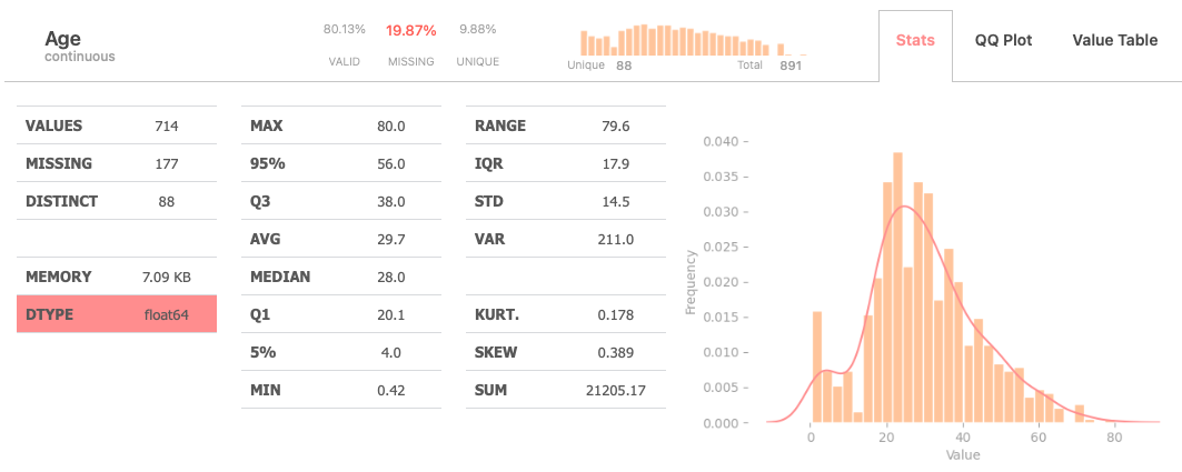
The “Stats” tab provides users with an extensive set of statistics
Additionally, the tab includes a histogram paired with a Kernel Density Estimation (KDE) plot, providing a comprehensive visualization of the variable’s distribution.
| VALUES | Number of valid values in the variable |
| MISSING | Number of missing observations in the variable |
| DISTINCT | Number of unique observations in the variable |
| MEMORY | Memory size of the variable |
| DTYPE | Pandas datatype |
| MAX | Maximum value of the variable |
| 95% | Value at the 95th percentile of the variable |
| Q3 | Third quartile (75th percentile) of the variable |
| AVG | Average (mean) value of the variable |
| MEDIAN | Median value of the variable |
| Q1 | First quartile (25th percentile) of the variable |
| 5% | Value at the 5th percentile of the variable |
| RANGE | Difference between maximum and minimum values |
| IQR | Interquartile Range - Difference between the first and third quartiles |
| STD | Standard deviation of the variable |
| VAR | Variance of the variable |
| KURT. | Kurtosis (measure of the “tailedness” of the distribution) of the variable |
| SKEW | Skewness (measure of asymmetry) of the variable |
| SUM | Sum of all values in the variable |
QQ Plot
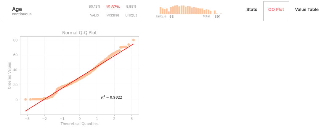
The tab features a QQ plot, which offers a graphical assessment of whether the data follows a theoretical normal distribution by comparing the quantiles of the variable against those of a theoretical distribution.
Value Table
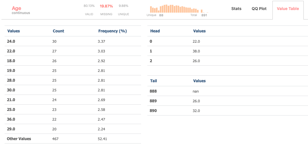
The value table organizes data by sorting values according to their frequency of occurrence, enabling quick identification of the most common values (up to 10) within the dataset.
And additionaly displaying the top three and bottom three values for quick reference and analysis.